MST124 Unit 3 - Functions

Introduction

Whenever one quantity depends on another, we say that the first quantity is a function of the second quantity.

1 Functions and their graphs

1.1 Sets of real numbers

A set is a collection of objects. The objects could be anything at all. An element or member is each of the objects in a set. Elements of the set belong to or are in a set.

A set can be specified by enclosing a list of elements in curly brackets, e.g.: $$ S = {5, 12, 34, 58} $$

A set can be described, e.g.: Let $T$ be the set of all odd integers. Sets are usually denoted with capital letters.

Empty set is denoted with $ \emptyset$. $\in$ means is in and $\notin$ means is not in.

An intersection is a process of forming new set out of overlapping members of two or more sets and is denoted as $A \cap B$.

Union is a process of forming new set out of all the members of two or more sets and is denoted as $A \cup B$.

$A$ is a subset of $B$ when every element of $A$ is also an element of $B$. A subset is denoted as $A \subseteq B$. Every set is a subset of itself and the empty set is a subset of every set.

The set of all real number is denoted as $\mathbb{R}$.

An interval is a set of real numbers that correspond to a continuous section of number line.

An endpoint is a number that lies at the end of an interval. The whole set of real numbers $\mathbb{R}$ is an interval with no endpoints.

Closed is such interval that includes all of its endpoints. Open interval doesn't include any of its endpoints. Half-open interval includes only one of its endpoints.

$\mathbb{R}$ doesn't have endpoints, so it's both open and closed.

Inequality signs can be used to describe intervals.

Interval notation can also describe intervals e.g.: $$ 4 \le x < 7 $$ is denoted as: $$ [4, 7) $$

An interval that extends indefinitely is denoted by $\infty$ or $-\infty$.

Union of intervals can be described as e.g.: $$ (-\infty, 2] \cup [4, 6) $$

1.2 What is a function?

A function consists of:

• a set of allowed input values, called the domain of the function
• a set of values in which every output value lies, called the codomain of the function
• a process, called the rule of the function, for converting each input value into exactly one output value.

A function can be denoted with function notation, e.g.: $$ h(x) = x^2 $$

The image set is a set of values in the codomain that do occur as output values.

Every value in the domain of a function must have exactly one output value.

If $f$ is a function, and $x$ is any value in its domain, then the value $f(x)$ is called the image of $x$ under $f$, or the value of $f$ at $x$, or $f$ maps $x$ to $f$.

Real functions have domain and codomain consisting of real numbers.

1.3 Specifying functions

Function specification consists of its domain and rule, e.g.: $$ f(x) = x^{2}+ 1 ~~ (0 \le x \le 6) $$ or

$$ f(x) = x^{2}+ 1 ~~ (x \in [0, 6]) $$

When a function is specified by just a rule, it's understood that the domain of the function is the largest possible set of real numbers for which the rule is applicable.

1.4 Graphs of functions

is the set of points $(x, y)$ in the coordinate plane such that $x$ is in the domain of $f$ and $y = f(x)$.

Functions increasing or decreasing on an interval

A function $f$ is increasing on the interval $I$ if for all values $x_1$ and $x_2$ in $I$ such that $x_1 < x_2$, $$ f(x_1) < f(x_2) $$

A function $f$ is decreasing on the interval $I$ if for all values $x_1$ and $x_2$ in $I$ such that $x_1 < x_2$, $$ f(x_1) > f(x_2) $$ (The interval $I$ must be part of the domain of $f$.)

1.5 Image sets of functions

In the same way as a domain of function can be visualized on the $x$-axis the image set of a function can be visualized on the $y$-axis.

The image set consists of all the possible output numbers, that is, all the points on the $y$-axis that lie directly to the right or left of a point on the graph.

1.6 Some standard types of functions

• Linear functions - has the rule of the form $f(x) = mx + c$.
• Constant function - a linear function whose rule is of the form $f(x) = c$.
• Quadratic functions - has the rule of the form $f(x) = ax^{2} + bx + c$.

Polynomial functions

Linear and quadratic functions are particular types of polynomial functions. Other example of polynomial function is: $$ f(x) = 2x^{4} - 5x^{3} + x^{2} + 2x - 3 $$

In general, a polynomial expression in $x$ is any expression that is a sum of finitely many terms, each of which is of the form $ax^{n}$ where $a$ is a number and $n$ is a non-negative integer.

Degree of a polynomial expression or function is the highest power of the variable $x$ in it.

Quadratic functions are polynomial functions of degree 2.

Linear functions are polynomial functions of degree 1, 0 or no degree at all.

Polynomial functions of degrees 3, 4, and 5 are called

• cubic
• quartic
• quintic

functions, respectively

Every polynomial function (with domain $\mathbb{R}$) that isn't a constant function tends to infinity or tends to minus infinity at the left and right.

Dominant term is a term in a rule of function with the highest power of $x$ and it defines whether the function tends to infinity or minus infinity. It's called dominant because it outweights (dominates) the sum of the values taken by all other temrs for large values of $x$.

If the dominant term has a plus sign and

• contains an even power of $x$, then the graph tends to infinity at both ends.
• contains an odd power of $x$, then the graph tends to minus infinity at the left and to infinity at the right.

If the dominant term has a minus sign and

• contains an even power of $x$, then the graph tends to minus infinity at both ends.
• contains an odd power of $x$, then the graph tends to infinity at the left and to minus infinity at the right.

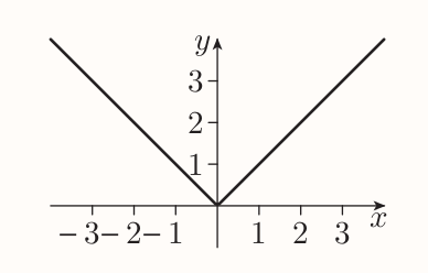
The modulus function

The modulus of a real number (or magnitude, absolute value) is its 'distance from zero' and for a real number $x$ its denoted as $|x|$.

THe modulus function is $$ f(x) = |x| $$

It follows form the definition that $$ \begin{equation*} |x| = \begin{cases} x \quad &\text{if} , x \ge 0 \ -x \quad &\text{if} , x < 0 \ \end{cases} \end{equation*} $$

So the graph of the modulus function is the same as the graph of $y = x$ when $x \ge 0$ and same as the graph of $y = -x$ when $x < 0$. It has a corner at the origin and image set of $[0, \infty)$.

The reciprocal function

If $x$ is any non-zero number, then the reciprocal of $x$ is $1/x$. The reciprocal function is $$ f(x) = \frac{1}{x} $$ With the domain of $(-\infty, 0) \cup (0, \infty)$.

It forms following graph

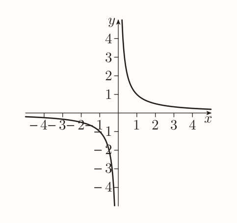
If a curve has a property when it gets arbitrarily close to straight line as it gets further away from origin then the straight line is called the asymptote of the curve.

Hence the coordinate axes are asymptotes of the graph of the reciprocal function.

Rational functions

The reciprocal and all polynomial functions are particular examples of rational functions.

The rational function is a function whose rule is of the form $$ f(x) = \frac{p(x)}{q(x)} $$ where $p$ and $q$ are polynomial functions.

f is polynomial function when $q$ is a constant function. f is a reciprocal function when $p(x) = 1$ and $q(x) = x$.

2 New functions from old functions

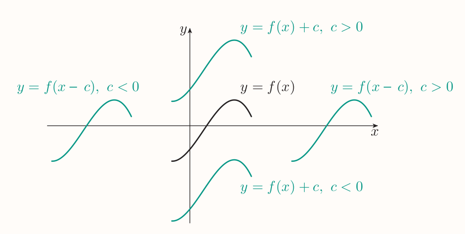
2.1 Translating the graphs of functions

A translation of a shape means sliding it to different position without rotating or reflecting it.

Suppose that $f$ is a function and $c$ is a constant. To obtain the graph of:

• $y = f(x) + c$, translate the graph of $y = f(x)$ up by $c$ units (the translation is down if $c$ is negative)
• $y = f(x - c)$, translate the graph of $y = f(x)$ to the right by $c$ units (the translation is to the left if $c$ is negative).

A translations can be combined. An equation $y = f(x)$ can be moved $c$ units to the right by replacing $x$ as $y = f(x - c)$. A shift up can be achieved by adding a constant $d$: $$ y = f(x - c) + d $$

Hence the original equation is translated to the right by $c$ units and up by $d$ units. Order of operations doesn't matter.

2.2 Scaling the graphs of functions vertically

Constant multiple is a function obtained by multiplying the RHS of a function rule by a constant, e.g. $g(x) = 8x^3$ is a constant multiple of the function $f(x)= x^3$.

The resulting effect on the graph of function is called the vertical scaling.

Vertical scaling of graphs

Suppose that $c$ is a constant. To obtain the graph of $y = cf(x)$, scale the graph of $y = f(x)$ vertically by a factor of $c$.

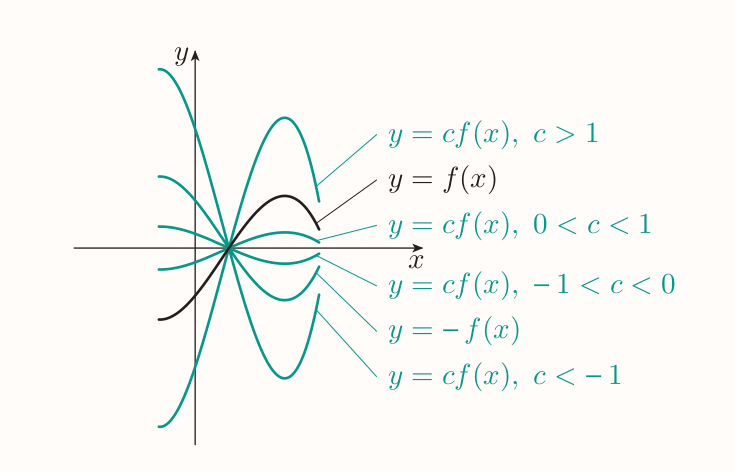
Negative of a function $f$ is the result of multiplying the right-hand side of the rule of a function $f$ by $-1$.

Vertical scaling can be combined with vertical and/or horizontal translations of graphs, e.g. $y = 4x^{3}+ 1$ scales the equation $y = x^3$ vertically by $4$ units, then translates it up by $1$ unit. The order of operations does often matter.

2.3 Scaling the graphs of functions horizontally

The horizontal scaling is achieved by replacing each occurrence of the input variable $x$ in the right-hand side of the rule of a function by an expression of the form $x/c$, where $c$ is constant.

The resulting effect on the graph of a function is called horizontal scaling.

Horizontal scalings of graphs

Suppose that $c$ is a non-zero constant. To obtain the graph of

$$ y = f(\frac{x}{c}) $$

scale the graph of $y = f(x)$ horizontally by a factor of $c$.

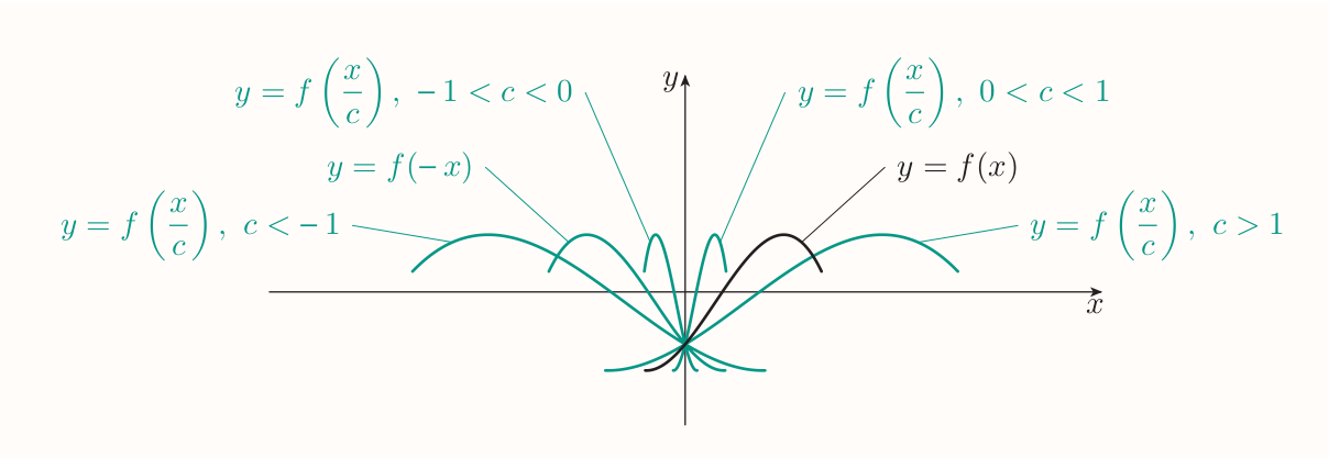
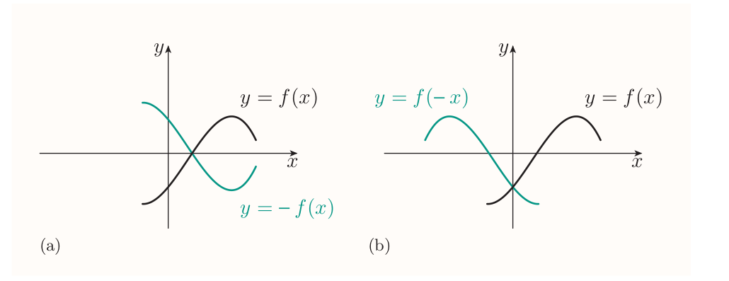
Reflections of graphs in the coordinate axes

To obtain the graph of $y = -f(x)$, reflect the graph of $y = f(x)$ in the $x$-axis. To obtain the graph of $y = f(-x)$, reflect the graph of $y = f(x)$ in the $y$-axis.

3 More new functions from old functions

3.1 Sums, differences, products and quotients of functions

Suppose that $f$ and $g$ are functions.

• The sum has the rule $h(x) = f(x) + g(x)$
• There are two differences
  • $h(x) = f(x) - g(x)$
  • $h(x) = g(x) - f(g)$
• The product has the rule $h(x) = f(x)g(x)$
• There are two quotients
  • $h(x) = \frac{f(x)}{g(x)}$
  • $h(x) = \frac{g(x)}{f(x)}$

3.2 Composite functions

Suppose $f$ and $g$, if the output of $f$ lies in the domain of $g$ it can be input to it.

A composite function is function whose rule is given by this process and whose domain is the largest set of real numbers to which you can apply the process. It's denoted by $g \circ f$ (the function that is applied first is second in the notation).

Definition of composite functions

Suppose that $f$ and $g$ are functions. The composite function $g \circ f$ is the function whose rule is $$ (g \circ f)(x) = g(f(x)) $$ and whose domain consists of all the values $x$ in the domain of $f$ such that $f(x)$ is in the domain of $g$.

The process of forming a composite function from two functions is called composing the functions. Functions $f$ and $g$ have two composite functions

• $g \circ f$, meaning apply $f$ first, than $g$
• $f \circ g$, meaning apply $g$ first, than $f$

3.3 Inverse functions

The inverse function of a function $f$, which is denoted by $f^{-1}$, is the function whose mapping diagram is obtained by reversing the direction of all the arrows in this full version of diagram.

One-to-one functions

A function $f$ is one-to-one if fo all values $x_1$ and $x_2$ in its domain such that $x_1 \ne x_2$, $$ f(x_1) \ne f(x_2) $$

Only one-to-one functions have inverse functions. Invertible function is a function that has an inverse function.

Definition of inverse functions

Suppose that $f$ is one-to-one function, with domain $A$ and image set $B$. Then the inverse function, or simply inverse, of $f$, denoted by $f^{-1}$, is the function with domain $B$ whose rule is given by $$ f^{-1}(y) = x, ~~~~~\text{where} ~~ f(x) = y $$ The image set of $f^{-1}$ is $A$.

Strategy to find the rule of the inverse function of a one-to-one function $f$

• Write $y = f(x)$ and rearrange this equation to express $x$ in terms of $y$.
• Use the resulting equation $x = f^{-1}(y)$ to write down the rule of $f^{-1}$. (Usually, change the input variable from $y$ to $x$.)

If a function is either increasing on its whole domain, or decreasing on its whole domain, then it is one-to-one and so has an inverse function.

For any pair of inverse functions $f$ and $f^{-1}$,

• $(f^{-1} \circ f)(x) = x$, for every value $x$ in the domain of $f$, and
• $(f \circ f^{-1})(x) = x$, for every value $x$ in the domain of $f^{-1}$

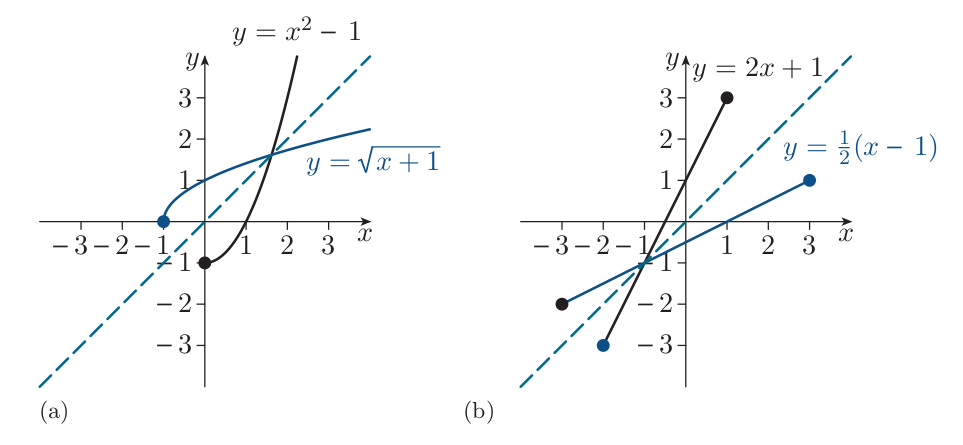
Graphs of inverse functions

The graphs of a pair of inverse functions are the reflections of each other in the line $y = x$ (when the coordinate axes have equal scales).

Functions that aren't one-to-one

Starting with a function $f$ that is not one-to-one, specify a new function that has same rule as $f$, but a smaller domain with following conditions satisfied:

• the new function is one-to-one and therefore has an inverse
• the image set of the new function is the same as the image set of the original function

E.g. for $f(x) = x^{2}$ the new function can be $g(x) = x^{2} ~~ (x \in [0, \infty))$. $g$ is one-to-one with inverse $g^{-1}(x) = \sqrt{x}$.

A function like $g$ that is obtained from another function $f$ by removing some numbers from its domain and keeping the rule is called a restriction of the original function $f$.

4 Exponential functions and logarithms

4.1 Exponential functions

Is a function whose rule is of the form $$ f(x) = b^x $$ where $b$ is a positive constant, not equal to 1. $b$ is called the base number of the exponential function.

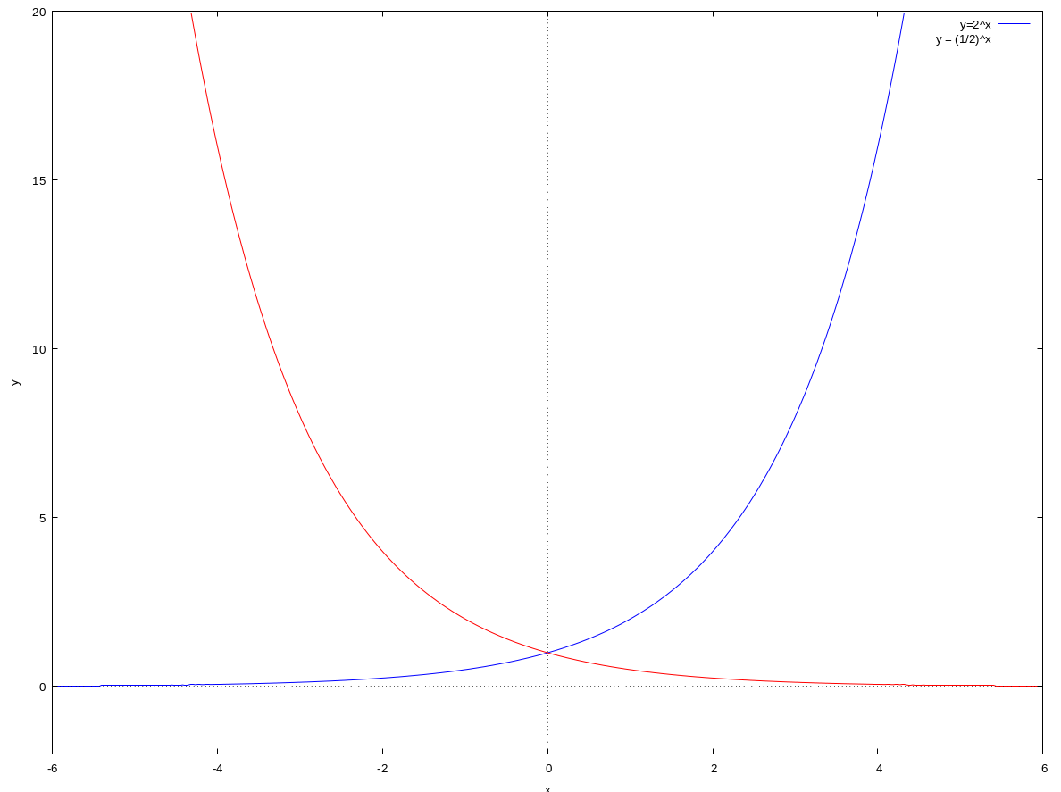
Graphs of exponential functions

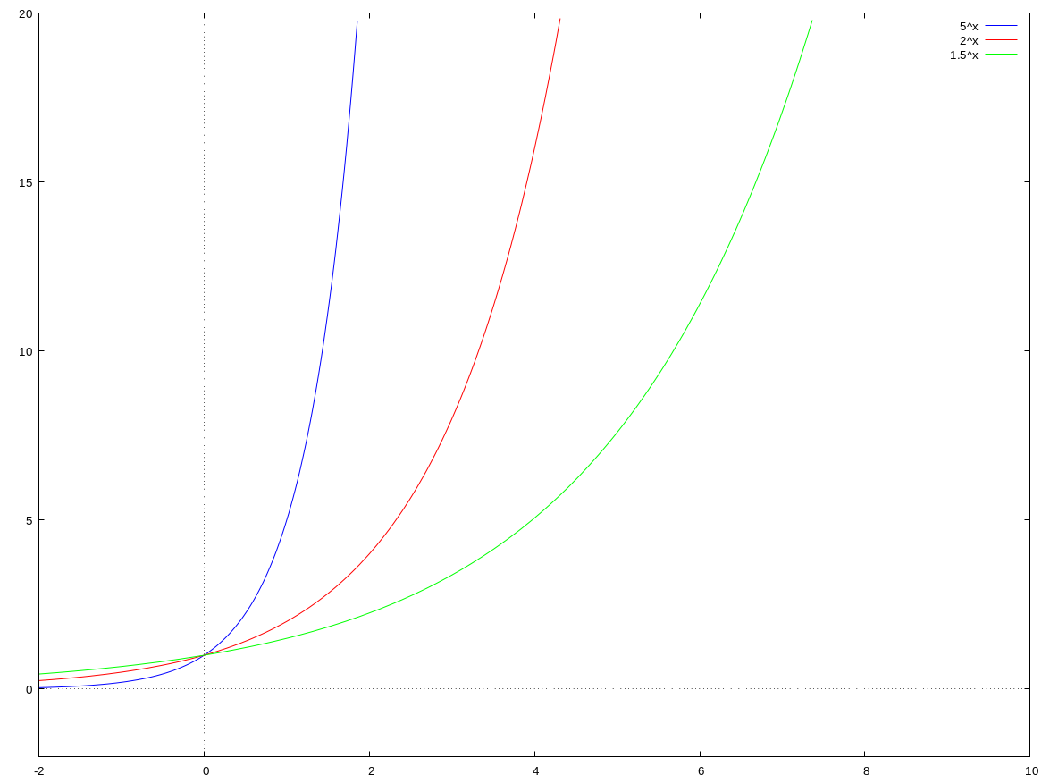
The graph of the function $f(x) = b^{x}$, where $b > 0$ and $b \ne 1$, has the following features.

• The graph lies entirely above the $x$-axis.
• If $b > 1$, then the graph is increasing, and it gets steeper as $x$ increases.
• If $0 < b < 1$, then the graph is decreasing, and it gets less steep as $x$ increases.
• The $x$-axis is an asymptote.
• The $y$-intercept is 1.
• The closer the value of $b$ is to 1, the flatter is the graph.

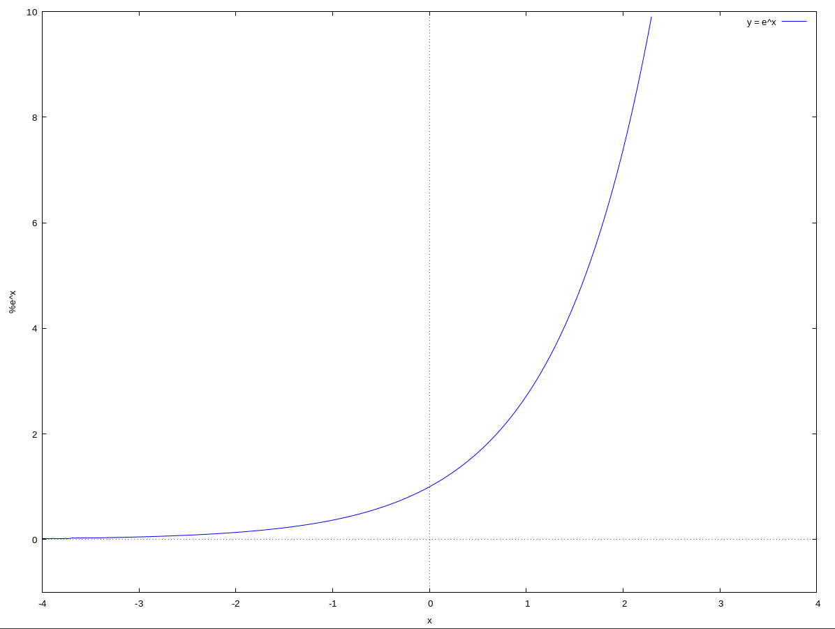
The exponential function

The graph of every exponential function $f(x) = b^{x}$ passes through the point $(0, 1)$. And its steepness depends on the value of $b$.

The exponential function with rule $f(x) = e^{x}$ has the special property that its gradient is exactly 1 at the point $(0,1)$, this function is referred to as the exponential function.

4.2 What is a logarithm?

Logarithms have a particular base Logs to base 10 are known as common logarithms with following definition. The logarithm to base 10 of a number $x$ is the power to which 10 must be raised to give the number $x$. e.g.: $$ \begin{align} \log_{10}100 = 2 \\[0.6em] \log_{10}1000 = 3 \\[0.6em] \log_{10}(\frac{1}{10})= -1 \end{align} $$

General definition of logarithms

The logarithm to base $b$ of a number $x$, denoted by $\log_bx$, is the power to which the base $b$ must be raised to give the number $x$. So the two equations $$ y = \log_bx ~~~ \text{and} ~~~ x = b^y $$ are equivalent. Remeber that:

• the base $b$ must be positive and not equal to 1
• only positive numbers have logarithms, but logarithms themselves can be any number.

Logarithm of the number 1 and logarithm of the base

For any base $b$, $$ \log_b1 = 0 ~~~ \text{and} ~~~ \log_bb = 1 $$

The most common bases of logarithms are $2$, $10$ and $e$. Logarithms to the base $e$ are called natural logarithms and the notation $\ln$ is often used.

Natural logarithms

The natural logarithm of a number $x$, denoted by $\ln x$, is the power to which the base $e$ must be raised to give the number $x$. So the two equations $$ y = \ln x ~~~\text{and} ~~~ x = e^y $$ are equivalent. Natural logarithms share following properties with common logs $$ \ln 1 = 0 ~~~ \text{and} ~~~ \ln e = 1 $$

4.3 Logarithmic functions

Are functions with a rule of the form $$ f(x) = \log_b x $$ where $b$ is a positive constant, not equal to 1.

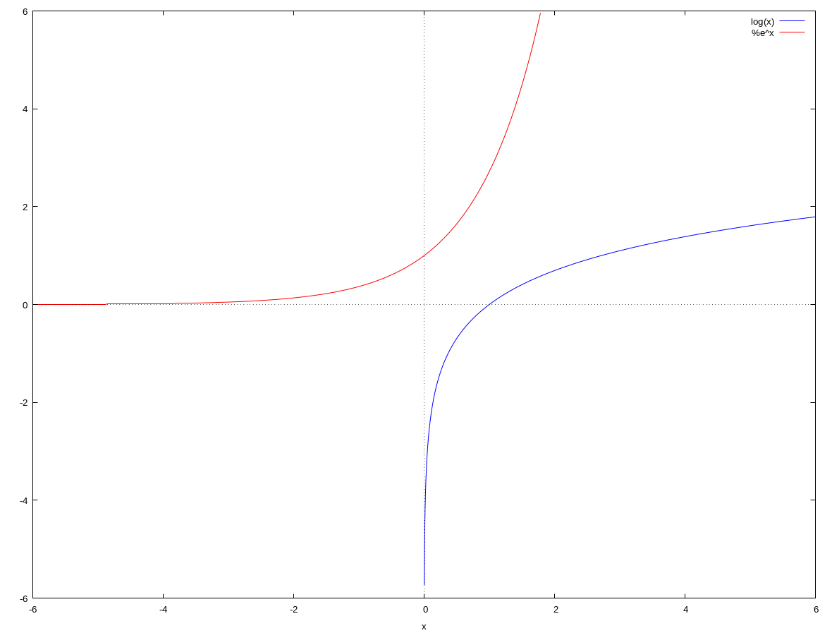
The logarithmic function $f(x) = \log_b x$ is the inverse function of the exponential function $g(x) = b^x$ since $$ y = \log_bx ~~~ \text{and} ~~~ x = b^y $$ are rearrangements of each other. Hence the graphs of both functions are reflections of each other in the line $y = x$.

Graphs of logarithmic functions

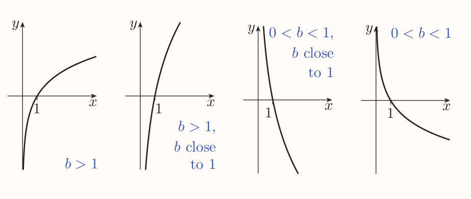
The graph of the function $f(x) = \log_bx$, where $b > 0$ and $b \ne 1$, has the following features.

• The graph lies entirely to the right of the $y$-axis.
• If $b > 1$, then the graph is increasing, and it gets less steep as $x$ increases.
• If $0 < b < 1$, then the graph is decreasing, and it gets less steep as $x$ increases.
• The $y$-axis is an asymptote.
• The $x$-intercept is 1.
• The closer the value of $b$ is to 1, the steeper is the graph.

For any base $b$, $$ \log_b(b^{x})= x ~~~ \text{and} ~~~ b^{\log_bx} = x $$ In particular, $$ \ln(e^{x}) = x ~~~ \text{and} ~~~ e^{\ln x} = x $$ (A composition of $f(x) = b^{x}$ and $f^{-1}(x) = \log_bx$)

4.4 Logarithm laws

Three logarithm laws

$$ \begin{aligned} \log_bx + \log_by = \log_b(xy) \\[0.5em] \log_bx - \log_by = \log_b(\frac{x}{y}) \\[0.5em] r\log_bx = log_b(x^r) \end{aligned} $$

Solving exponential equations

An exponential equation has the unknown in the exponent, e.g. $$ 5^{x}= 130 $$

And the third logarithm law can be used to solve those. It's useful to swap the sides for this purpose: $$ \log_b(x^{r)}= r\log_b(x) ~~~ \text{in particular} ~~~ \ln(x^{r}) = r\ln(x) $$

4.5 Alternative form for exponential functions

Any exponential function $f(x) = b^x$, where $b$ is a positive constant not equal to 1, can be written in the alternative form $$ f(x) = e^{kx} $$ where $k$ is a non-zero constant. The constant $k$ is given by $k = \ln b$.

This fact gives following alternative definition of an exponential function An exponential function is a function whose rule is of the form $$ f(x) = e^{kx} $$ where $k$ is a non-zero constant. And properties of exponential graphs can be rewritten as

Graphs of exponential functions

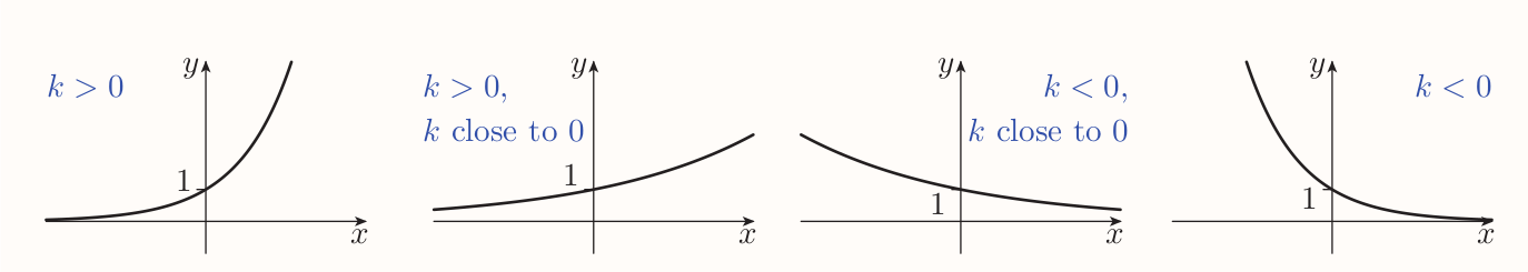
The graph of the function $f(x) = e^{kx}$, where $k \ne 0$, has the following features.

• The graph lies entirely above the $x$-axis.
• If $k > 0$, then the graph is increasing, and it gets steeper as $x$ increases.
• If $k < 0$, then the graph is decreasing, and it gets less steep as $x$ increases.
• The $x$-axis is an asymptote.
• The $y$-intercept is 1.
• The closer the value of $k$ is to 0, the flatter is the graph.

The graph of every exponential function is a horizontal scaling of the graph of the exponential function $f(x) = e^x$.

4.6 Exponential models

Are defined by a function with rule of the form $f(x) = ab^{x}$. That is equal to $f(x) = ae^{kx}$ in the alternative form.

$f(x) = ae^{kx}$ is obtained by

• vertically scaling the graph of the function $g(x) = e^{kx}$ by the factor of $a$.

$g(x) = e^{kx}$ is obtained by

• horizontally scaling the graph of the function $h(x) = e^{kx}$ by a factor of $1/k$.

Hence the graph of the function $f(x) = ae^{kx}$ is obtained by scaling the graph of the function $h(x) = e^x$ both horizontally and vertically.

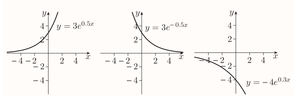
A quantity is changed exponentially when the change can be modeled by a function with rule of the the form $f(x) = ae^{kx}$.

If $a$ and $k$ are positive then the quantity is said to grow exponentially and the function is called exponential growth function.

If $a$ is positive but $k$ is negative then it's said the quantity decays exponentially, the function is exponential decay function and graph is called an exponential decay curve.

A characteristic property of exponential growth and decay functions

If $f(x) = ae^{kx}$, then whenever $p$ units are added to the value of $x$, the value of $f(x)$ is multiplied by $e^{kp}$

The reason is following. Say the value of $x$ changes from $$ f(x) = ae^{kx} ~~~ \text{to} ~~~ f(x + p) = ae^{k(x + p)} $$ Then $$ ae^{k(x + p)} = a^{kx + kp} = ae^{kx}e^{kp} = f(x) \times e^{kp} $$

The factor by which $f(x)$ is multiplied is called growth or decay factor.

• Growth factors are $> 1$
• Decay factors are between 0 and 1, exclusive.

Doubling and halving periods

Suppose that $f$ is an exponential growth function. Then $p$ is the doubling period of $f$ if whenever you add $p$ to $x$, the value of $f(x)$ doubles.

Similarly, suppose that $f$ is an exponential decay function. Then $p$ is the halving period of $f$ if whenever you add $p$ to $x$, the value of $f(x)$ halves.

Strategy to find a doubling or halving period

If $f(x) = ae^{kx}$ is an exponential growth function (so $k > 0$), then the doubling period of $f$ is the solution $p$ of the equation $e^{kp} = 2$; that is, $p = (\ln2)/k$.

Similarly, if $f(x) = ae^{kx}$ is an exponential decay function (so $k < 0$), then the halving period of $f$ is the solution $p$ of the equation $e^{kp} = \frac{1}{2}$; that is, $p = \ln \frac{1}{2}/k= -(\ln 2)/k$.

5 Inequalities

5.2 Rearranging inequalities

Carrying out any of the following operations on an inequality gives an equivalent inequality.

• Rearrange the expressions on one or both sides.
• Swap the sides, provided you reverse the inequality sign.
• Do any of the following things to both sides:
  • add or subtract something
  • multiply or divide by something that's positive
  • multiply or divide by something that's negative, provided you reverse the inequality sign.

Both sides shouldn't be multiplied by a variable unless it's limited o positive values only.